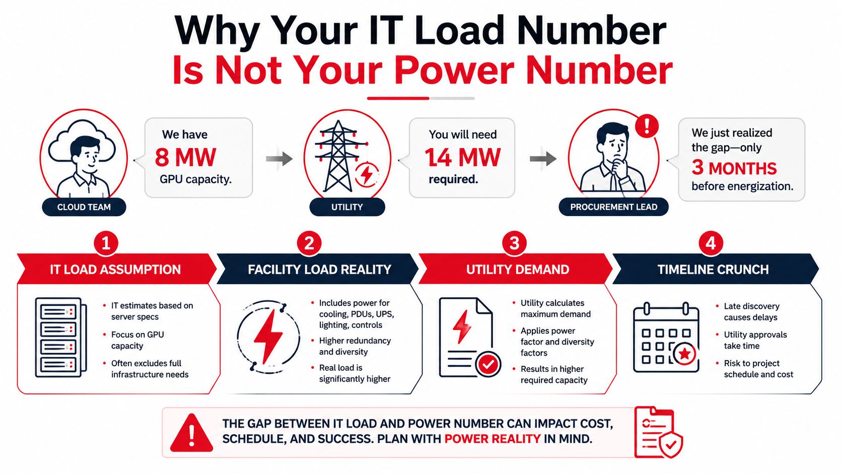
A cloud team announces 8 MW of new GPU capacity, and everyone initially treats that figure as the project's power requirement. Then the utility asks for 14 MW, the electrical engineer revises the UPS and generator schedule, and the procurement lead discovers the gap only three months before energization. The problem isn't that anyone misread a server specification. The problem is that an IT load is only the first number in a much longer chain.
Data center power requirements connect compute demand to facility systems, utility service, backup generation, cooling, redundancy, and construction timing. A sound capacity model therefore answers two questions at once: How much power will the equipment need, and can the site secure and deliver that power when the project needs it?
Why Your IT Load Number Is Not Your Power Number
A project team may approve an 8 MW IT load and still face a larger utility request, a different equipment schedule, and a later energization date. The IT figure covers electricity used by servers, storage, and networking equipment. It leaves out UPS and distribution losses, cooling, pumps, lighting, controls, security systems, and capacity reserved for future deployment.
The gap affects procurement as much as engineering. A utility evaluates the service entrance, transformers, medium-voltage feeders, substations, protection equipment, operating limits, and expected demand profile. The facility designer must size switchgear, UPS modules, generators, busways, cooling equipment, and distribution paths for normal operation and failure scenarios. Each choice can create a longer lead time or require a larger interconnection request.
The conversion chain
Build the capacity model in layers:
- IT load: Server, storage, and network consumption.
- Critical load: IT equipment plus systems that must remain supported during a utility interruption.
- Facility load: Critical load plus cooling, electrical losses, lighting, controls, and other building services.
- Utility demand: Metered service capacity, including operating margin, staged growth, and the site's demand profile.
Power Usage Effectiveness, or PUE, connects IT consumption with total facility power:
PUE = total facility energy ÷ IT energy
A PUE of 1.43 means each unit consumed by IT requires about 1.43 units for the whole facility. Applied to an 8 MW IT assumption, that produces roughly 11.44 MW before redundancy, growth, and other design decisions. It is a planning conversion, not a complete utility-interconnection value.
The schedule must be modeled alongside the arithmetic. The International Energy Agency's analysis of energy demand from AI estimates global data center electricity consumption at about 415 TWh in 2024, or roughly 1.5% of worldwide electricity use, and projects about 945 TWh by 2030. That scale helps explain why a utility may treat a data center as a major power-system project. If permanent capacity will arrive in stages, document temporary generation, hybrid power staging, and the headroom needed for later racks before placing equipment orders.
Practical rule: Freeze the assumptions behind the load number before requesting a utility commitment. A change in rack count, density, cooling method, or redundancy can alter the interconnection request, equipment procurement, and energization date.
The Language of Data Center Power
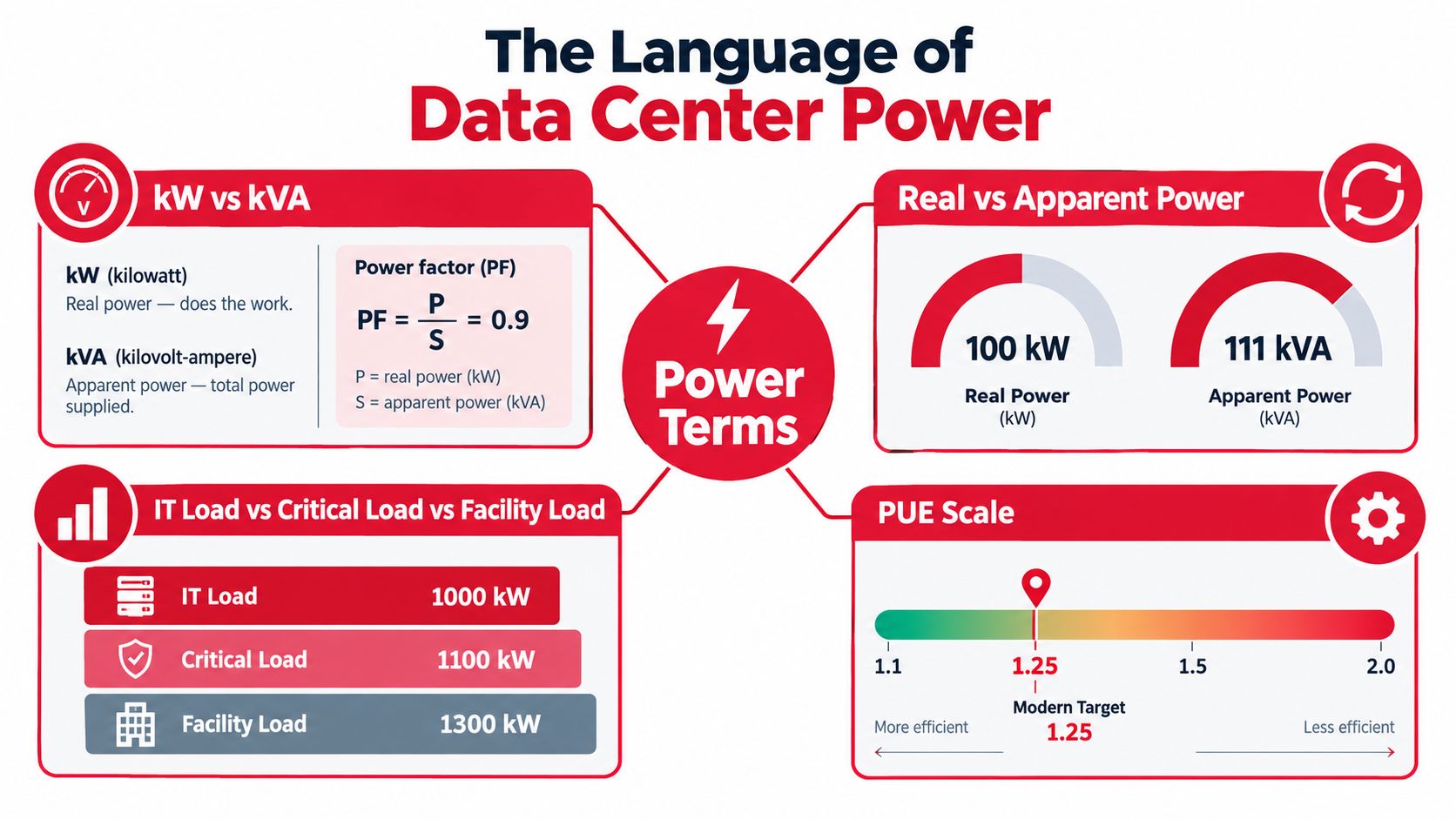
A capacity model can look complete while mixing unlike quantities. kW measures real power doing useful work, like water reaching a machine. kVA measures apparent power, the electrical carrying capacity required by the equipment, like the pipe sized to deliver that flow.
Power factor explains the gap. A load with a power factor of 0.9 requires more apparent capacity than its real-power figure suggests:
kVA = kW ÷ power factor
A 900 kW load at a 0.9 power factor therefore requires about 1,000 kVA of apparent capacity. Final equipment selection still depends on voltage, harmonics, transient behavior, manufacturer data, and applicable engineering standards. Keeping kW and kVA separate prevents a sizing error that can affect transformers, switchgear, UPS systems, and the utility request.
Three load categories
IT load is the computing equipment itself. Critical load includes IT equipment plus the electrical systems that must continue through a disruption, such as selected controls, monitoring, and cooling equipment. Facility load covers the building's full normal operating demand, including mechanical systems and electrical losses.
Capacity documents also use “capacity” in three different ways:
- Nameplate capacity: The rating printed on equipment or provided by the manufacturer. It can exceed normal operating demand.
- Design capacity: The load used to size infrastructure under defined operating conditions.
- Provisioned capacity: The amount installed, energized, or made available for a customer or IT deployment.
A simple worked example
Assume an IT load of 1,000 kW and a facility PUE of 1.43:
1,000 kW × 1.43 = 1,430 kW
The modeled facility load is therefore approximately 1.43 MW. That figure supports early procurement and utility discussions, but it does not select the UPS topology, generator fleet, utility service, or expansion allowance. Each decision changes equipment quantities, lead times, commissioning work, and sometimes the required interconnection.
Industry planning conventions place average data centers commonly in the 5 to 10 MW range, while large hyperscale facilities increasingly require 100 MW or more. These scales create different procurement and schedule problems. A smaller site may fit within an existing service strategy, while a large campus can require major substation work and a longer utility review. If the permanent supply will arrive in stages, model temporary generation, hybrid power staging, and headroom for later racks before ordering long-lead equipment.
Sizing IT Load by Facility Scale and Density
Facility scale gives you a starting point, but rack density determines how the load behaves inside the building. Two sites can have the same total IT demand and require very different busways, cooling systems, floor layouts, branch circuits, and commissioning plans.
The table below is a planning framework, not a substitute for an equipment schedule. The facility categories and density ranges in the planning notes are useful for orientation, while the Uptime Institute's 2026 Global Data Center Survey reports that the average of modal rack densities surpassed 11 kW for the first time.
| Facility Tier | Typical IT Load | Rack Density Range | Recommended Design Headroom |
|---|---|---|---|
| Enterprise edge or equipment room | Under 50 kW | 4 to 12 kW | Reserve panel and cooling capacity for expected equipment additions |
| Regional colocation room | 1 to 5 MW | 4 to 20 kW | Provide flexible distribution and space for denser customer deployments |
| Enterprise or hyperscale hall | 20 to 100 MW | 10 to 30 kW | Reserve electrical and cooling paths for phased hall growth |
| AI or HPC campus | Beyond 250 MW per building | 60 to 130 kW for GPU-oriented racks | Design the power, liquid cooling, and utility strategy around future compute blocks |
Density changes the building
General-purpose compute may fit comfortably within moderate rack densities. Dense storage and GPU systems push more current through the rack, increase heat rejection, and may require different busway ratings and liquid-cooling provisions. The 2025 Uptime Institute survey places the average of modal densities near 9 kW and notes that average server-rack densities remain concentrated in the 10 to 30 kW band, with few facilities exceeding 30 kW.
That distribution supports a practical design position. Most new facilities shouldn't assume every rack will become an extreme-density AI rack, but they also shouldn't lock themselves into an architecture that can't support denser equipment later. A flexible electrical design may use reserved busway positions, spare transformer capacity, adaptable branch distribution, and cooling zones that can be upgraded without dismantling an operating hall.
For feeder, panel, and branch-circuit calculations, planners can use NEC-aligned load formulas as a reference point, then validate the result against the project's equipment schedules and local requirements.
Design decision: Headroom isn't an arbitrary cushion added at the end. It's a deliberate reservation for equipment density, workload changes, cooling retrofits, and the time required to obtain new electrical capacity.
Converting IT Load into Real Facility Power
A site planned around 2 MW of IT load may still need more than 3 MW of utility capacity once losses, cooling, operating margin, and future deployment are included. Treat the calculation as a procurement model, not a watts-on-paper exercise. Each multiplier affects the service request, equipment orders, interconnection timeline, and room for later expansion.
A useful model keeps those assumptions visible:
Facility kW = IT kW × distribution-loss factors × PUE × safety factor × growth factor
When losses are represented through efficiency divisions, use:
IT kW × 1 ÷ efficiency factors × PUE × safety factor × growth factor
The inputs must match the design basis. PDU efficiency may fall in the 96% to 98% range, while busway efficiency may be about 99%. A planning safety factor of 1.1 can apply when supported by the engineering basis. A growth factor of 1.2 to 1.5 can be reasonable when tied to a documented deployment schedule. It should not be a placeholder chosen without a load plan.
A 2 MW example
Assume 2 MW of IT load, a PUE of 1.25, distribution efficiencies of 96% and 99%, a 1.1 safety factor, and a growth factor between 1.2 and 1.5.
The resulting utility requirement is approximately 2.6 MW to 3.3 MW, depending on rounding and how the project treats losses. A narrower estimate of roughly 2.6 to 3.1 MW may result when the loss assumptions and operating margin are defined differently. The sequence matters more than false precision. The utility service requirement is materially higher than the initial IT figure.
That growth allowance covers more than additional cabinets. It may support hot-aisle containment retrofits, GPU densification, changing workload mixes, and the capacity needed to avoid an early breaker, transformer, or UPS upgrade. It also affects procurement timing. A larger service request may require utility studies, new interconnection equipment, or a longer delivery path than the original IT schedule suggests.
Model the equipment chain separately
Use the facility requirement to test each part of the power path:
- Utility service: Normal demand, contracted capacity, fault contribution, and future expansion.
- UPS plant: Critical-load support, module loading, bypass arrangements, battery systems, and redundancy.
- Generators: Backup capacity, starting sequence, step-load response, fuel systems, and emissions requirements.
- Distribution: Medium-voltage equipment, transformers, switchgear, busways, panelboards, and branch circuits.
The broader AI demand trend reinforces the need for a credible forecast. A project's growth factor should still come from its deployment schedule, rack strategy, and cooling plan. Utilities will examine that forecast when deciding whether the requested capacity and expansion phases are feasible.
A hybrid power plan can stage capacity as the site grows, pairing an initial utility block with defined future service upgrades or temporary generation where appropriate. The right answer depends on interconnection timing, equipment lead times, and the cost of carrying unused headroom. Document those trade-offs before placing long-lead orders.
Choosing the Right Redundancy Topology
Redundancy is a capacity-versus-risk decision. N means the installed system can carry the required load with no spare module. N+1 adds one module beyond the calculated requirement. 2N provides two complete capacity paths, and 2N+1 adds a spare module to each of those paths or to the defined redundant arrangement.
Consider a 5 MW critical load:
| Topology | Nameplate for 5 MW IT | Maintainability | Typical Use |
|---|---|---|---|
| N | 5 MW | Planned maintenance may require a transfer or outage strategy | Smaller or less critical installations |
| N+1 | 6 MW | One module can be unavailable while the remaining system carries the load | Colocation and hyperscale environments |
| 2N | 10 MW | One full path can be maintained or lost while the other supports the load | High-criticality financial or healthcare operations |
| 2N+1 | 11 MW | One path remains resilient with additional module margin | Facilities with very stringent availability objectives |
The arithmetic is straightforward, but the physical consequences are not. A 2N design for a 5 MW critical load commits the electrical plant to 10 MW of nameplate capacity before additional growth or facility loads. That commitment affects utility service, transformers, switchgear, UPS modules, generators, fuel systems, cooling, floor space, commissioning, and the amount of equipment that may sit lightly loaded.
Maintenance is part of the topology
Ask what the system must tolerate while maintenance is underway. If technicians need to remove a UPS module, breaker, generator, or cooling component without interrupting the critical load, the architecture must provide a safe alternate path and enough remaining capacity.
N+1 can provide concurrent maintenance when the switching, controls, and operating procedures are designed correctly. It isn't automatically maintainable because an extra module exists. Conversely, 2N can reduce dependence on a single path, but it introduces more equipment, more controls, more testing, and more opportunities for configuration errors.
Capacity choice: Select redundancy from the business consequence of an interruption, not from a generic ranking where 2N is always treated as “better.”
A planner should document the failure window, maintenance method, transfer sequence, and maximum permitted load on each surviving path. The answer may differ between an enterprise room, a customer-facing colocation hall, and a regulated clinical workload.
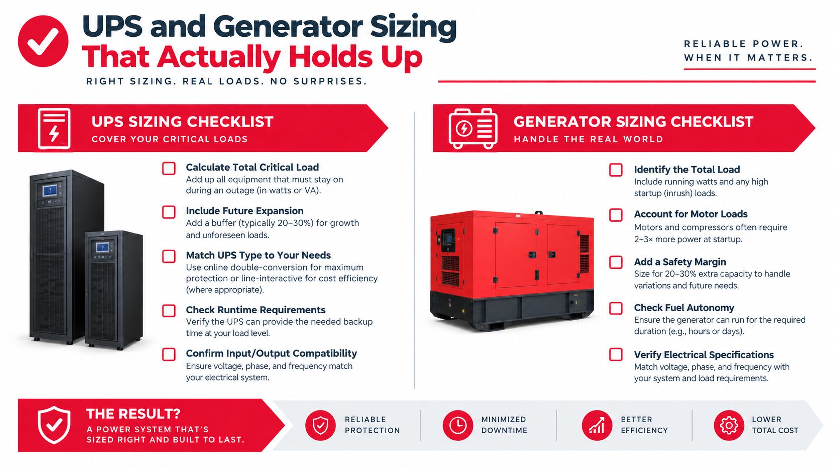
UPS and Generator Sizing That Actually Holds Up
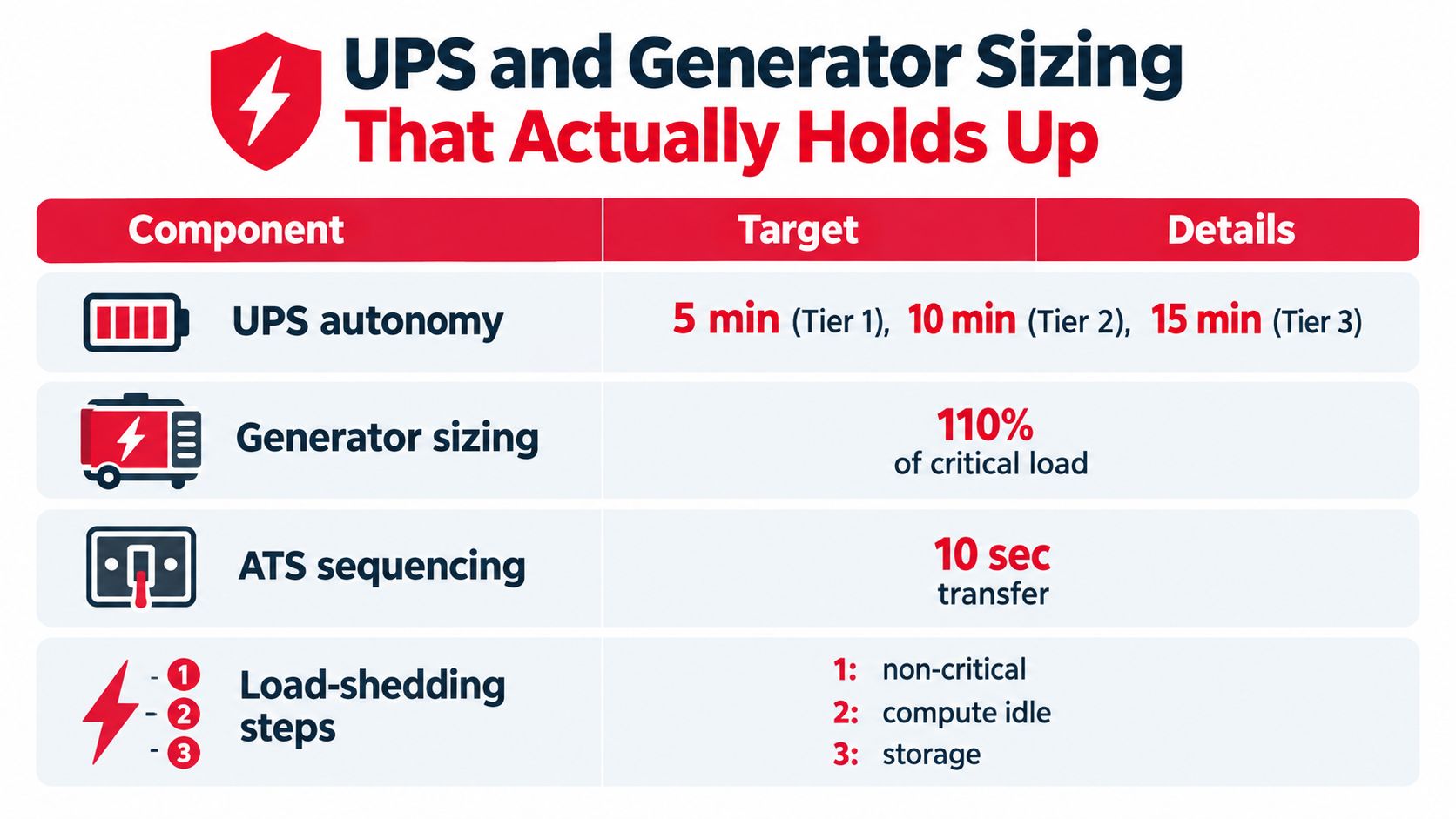
A backup plant works as a chain. The UPS bridges the interval between utility loss and generator availability. The generator then supports the critical load for the outage duration. Automatic transfer switches coordinate the source change, while load-shedding prevents nonessential equipment from destabilizing the system.
Start with the ride-through requirement
Battery autonomy should match the generator-start sequence and the site's risk tolerance. Planning targets may include 5 minutes for Tier 1, 10 minutes for Tier 2, and 15 minutes for Tier 3, as represented in the required sizing visual. Longer autonomy can make sense where fuel delivery, generator reliability, or utility restoration creates a credible need, but extra battery capacity adds cost, weight, space, maintenance, and replacement planning.
The UPS model must use the critical load, not the server nameplate total. Include the supported cooling and controls that must remain active, then apply the selected redundancy topology. An N+1 plant and a 2N plant don't use the same module count even when the protected IT load is identical.
Size generators for behavior, not just steady state
Generators must handle starting currents, UPS recharge, cooling motors, harmonic effects, and staged transfers. A generator bank that appears adequate at steady-state kW can still fail when multiple loads connect at once.
A sequence usually works like this:
- Detect the outage and start the generator.
- Transfer essential mechanical and electrical loads in stages.
- Hold noncritical loads until the source is stable.
- Add compute and storage loads according to the operating sequence.
- Shed lower-priority loads if the generator or fuel system approaches its limit.
Diesel systems require a fuel plan that covers storage, replenishment, testing, environmental controls, and delivery access. Natural-gas generation can support extended runtime without the same on-site liquid-fuel storage model, but it introduces dependence on the gas network and local permitting.
The IEA's reporting on data center electricity bottlenecks describes developers moving toward onsite generation when grid connections take too long. That choice can improve schedule certainty, but it shifts the project toward fuel contracts, emissions compliance, maintenance staffing, and community permitting.
Why Cooling Decisions Live Inside the Power Plan
Every watt delivered to a server eventually becomes heat that the facility must reject. Cooling therefore isn't a separate line item that can be finalized after the electrical design. The rack voltage, distribution arrangement, target density, inlet temperature, airflow strategy, and PUE assumption all influence the cooling plant and its parasitic power.
Conventional air cooling may work well for moderate rack densities. As density rises, fans move more air, containment becomes more important, and the facility may need rear-door heat exchangers, chilled-water systems, or direct-to-chip liquid cooling. Liquid systems can support dense compute, but they add pumps, heat exchangers, water-quality controls, leak detection, and maintenance procedures.
| Rack Density (kW) | Cooling Method | Typical kW Overhead per 100 kW IT Load | Notes |
|---|---|---|---|
| Below 15 | Conventional air | Project-specific | Standard airflow and containment may be sufficient |
| 15 to 30 | Hot-aisle or cold-aisle containment | Project-specific | Airflow management becomes central to usable capacity |
| 30 to 50 | Rear-door or hybrid cooling | Project-specific | Electrical and mechanical systems need coordinated zoning |
| Above 50 | Direct-to-chip or other liquid cooling | Project-specific | Pumps, heat exchangers, controls, and water management become part of the critical design |
The table intentionally avoids a universal overhead number. Cooling power varies with climate, set points, heat-rejection equipment, chilled-water temperature, economizer availability, redundancy, and operating mode. A higher chilled-water temperature may reduce compressor work in one design, while a different climate or control sequence changes the result.
Make the cooling topology explicit
Before finalizing the facility power number, identify:
- Heat-transfer path: Air, rear-door, direct-to-chip liquid, or a hybrid arrangement.
- Heat-rejection plant: Air-cooled, water-cooled, dry cooler, cooling tower, or another approved system.
- Operating envelope: Inlet temperature, humidity, ambient conditions, and equipment limits.
- Failure behavior: What cooling remains available after a pump, chiller, fan, or power path fails.
For planners building a detailed mechanical cost and capacity model, Exayard HVAC estimating software can help organize HVAC quantities and estimates alongside the project's engineering assumptions.
If you can't name the cooling topology, you can't defend the facility power number.
Scaling for Growth Without Rebuilding the Plant
A campus can have vacant floor space and spare cabinet positions yet remain unable to add IT load. The constraint is often the utility interconnection, followed by transformer availability, substation construction, medium-voltage feeder upgrades, transmission capacity, permitting, and the utility's construction schedule. For procurement planning, the contracted service date matters as much as the watts on the electrical one-line.
Data center demand is already material within major electricity markets, and grid capacity can limit expansion before the building is ready. Recent planning projections describe U.S. data center demand rising from 31 GW in 2025 to 41 GW in 2026 and 66 GW in 2027. Treat those figures as schedule pressure, not merely a load forecast. A delayed interconnection can hold the project longer than equipment installation or interior fit-out.
Stage the physical plant
A phased design preserves future options without energizing every block on day one:
- Build shell space early: Reserve rooms, clearances, cable routes, and equipment yards for later phases.
- Pre-stub distribution: Install or reserve busway routes and feeder positions so later deployment does not require major demolition.
- Use modular UPS blocks: Plan additions in repeatable capacity blocks, such as 250 kW modules where the equipment and operating model support them.
- Reserve equipment bays: Protect space for future transformers, generators, switchgear, fuel systems, and cooling equipment.
- Separate energized capacity from installed capacity: An empty equipment position does not equal contracted utility service.
A useful capacity model has two timelines. One tracks installed equipment. The other tracks what the utility, permits, and site infrastructure can deliver. The slower timeline sets the expansion date.
Treat hybrid power as a schedule tool
The 2026 Power Report from Bloom Energy reports that expectations for fully onsite-powered facilities increased by 22% in six months. It also describes hyperscale campuses requiring 200 MW to 500 MW, with a growing number of connection requests above 1,000 MW.
Those figures do not make onsite power suitable for every site. They do justify evaluating a hybrid arrangement in which utility service, onsite generation, battery storage, and staged IT deployment operate together. Onsite natural-gas generation or fuel cells may bridge an interconnection delay. Batteries can support short interruptions and transient demand. Each choice adds fuel, maintenance, emissions, permitting, controls, and operating risks, so compare those obligations with the utility upgrade schedule rather than treating generation as free capacity.
Procurement can control the project more tightly than land or capital. If the final service request waits until construction, the utility upgrade may become the schedule's controlling path.
Southern Tier Resources supports data center infrastructure fit-outs that integrate power, connectivity, and structured cabling. Its planning addresses day-one capacity and future high-density compute needs. Visit Southern Tier Resources to discuss phased deployment, from infrastructure planning and fit-out through testing and ongoing maintenance.