
Your business site passes its fiber speed test, yet video calls freeze every afternoon. The circuit stays up, the router shows no obvious fault, and the help desk keeps hearing that the internet is slow. Replacing equipment without measuring the failure would be an expensive guess.
Network performance metrics turn that complaint into a testable problem. The useful question isn't just how much traffic the connection can carry. It's whether packets arrive predictably, whether performance holds under load, and which segment stops meeting the application's needs.
Core Network Metrics at a Glance
A successful speed test proves that a particular endpoint delivered traffic over a particular path during that test. It doesn't prove that the same connection can support interactive applications during the afternoon rush.
Start with throughput, the data successfully delivered per second under load. Keep it separate from bandwidth, which describes the capacity available rather than the delivery achieved.
Latency measures delay. Operational dashboards commonly report round-trip time, or RTT, so label the direction explicitly rather than treating one-way delay and RTT as interchangeable.
Core network performance metrics and reference points
| Metric | What It Measures | Unit | Common Reference Point |
|---|---|---|---|
| Throughput | Data delivered per second under load | Mbps or Gbps | Compare against contracted or designed capacity |
| Latency | Round-trip time for a packet to reach a target and return | ms | Compare the same endpoints, direction, and load condition |
| Jitter | Variation in packet delay within the same flow | ms | Use the application's tolerance for delay variation |
| Packet loss | Share of test packets not delivered within the defined timeout | % | Set an application-specific ceiling and inspect loss bursts |
| Availability | Share of time the service is usable | % | Define usability and the reporting window before calculating |
| Utilization | Share of link capacity in use | % | Compare peak demand with queueing and discard behavior |
Jitter describes variation within a flow, not the difference between unrelated ping results. A call needs predictable packet delivery, while a bulk transfer can tolerate more variation.
Packet loss measures missing packets against packets sent. The timeout matters because a monitoring system must decide when a delayed packet becomes a lost packet.
Availability describes whether the service is usable over the reporting period. Utilization describes how much capacity traffic consumes, with upstream and downstream measured separately.
Establish a repeatable foundation
The FCC's Measuring Broadband America methodology centers on download and upload throughput, latency, and packet loss; its 2020 cycle sent approximately 2,000 latency-testing packets per hour at random intervals and classified packets not acknowledged within three seconds as lost.
That timeout is a measurement definition, not a statement that applications can tolerate the delay. A voice packet can arrive too late to be useful without meeting a test's definition of loss.
Use the full set to choose an investigation, not to generate a dashboard full of unrelated gauges. Match the complaint to the likely metric before touching equipment, then verify the suspected cause against neighboring measurements.
Why Speed Alone Misleads Network Teams
Think of throughput as the number of road lanes, latency as the trip duration, jitter as uneven stop-and-go progress, and packet loss as vehicles that never arrive. Adding lanes won't make a long, unpredictable journey feel responsive.
The traffic analogy helps separate capacity from timing.

Architecture changes responsiveness
The FCC's 2014 Measuring Broadband America report reported the following September 2013 peak-period RTT measurements and cited ITU guidance that one-way latency below 150 milliseconds may support many applications, while above 400 milliseconds is unacceptable for most broadband uses.
Peak-period round-trip latency by access technology, 2013
| Access Technology | Average Peak RTT | What It Shows |
|---|---|---|
| Fiber-to-the-home | 24 ms | Lowest measured latency of the terrestrial technologies |
| Cable | 32 ms | Mid-range responsiveness at peak hours |
| DSL | 49 ms | Highest latency of the three technologies at peak |
| All terrestrial technologies | 34.9 ms | Average up from 29.6 ms in February 2013 |
These historical results aren't current acceptance targets. They demonstrate that access architecture and path design affect responsiveness independently of the advertised speed tier.
Directionality also matters. Don't compare a ping RTT directly with a one-way application requirement, and don't assume halving RTT produces an accurate one-way measurement when the paths or queues are asymmetric.
Uneven delivery changes application behavior
A stable path lets a voice receiver use a predictable playout buffer. When packets arrive unevenly, the receiver may expand that buffer, adding delay to avoid gaps in the audio.
The IETF's RFC 7928 distinguishes delay variation from average delay and identifies queueing and processing variations as important contributors. That's why paths with similar average RTT can behave differently during a call.
Loss distribution matters too. In a hypothetical call, a cluster of consecutive missing packets can remove an audible stretch of speech, while the same number of losses scattered across a long session may be easier for the application to conceal.
This video offers another way to visualize the relationship between the measurements.
Practical rule: A throughput result establishes capacity under the test conditions. It doesn't establish predictable delivery.
Before approving an upgrade, distinguish a capacity shortage from a long path, unstable queue, or localized loss event. More bandwidth may relieve congestion, but it won't shorten an unnecessarily indirect route or repair a damaged optical connection.
How to Measure Network Performance Step by Step
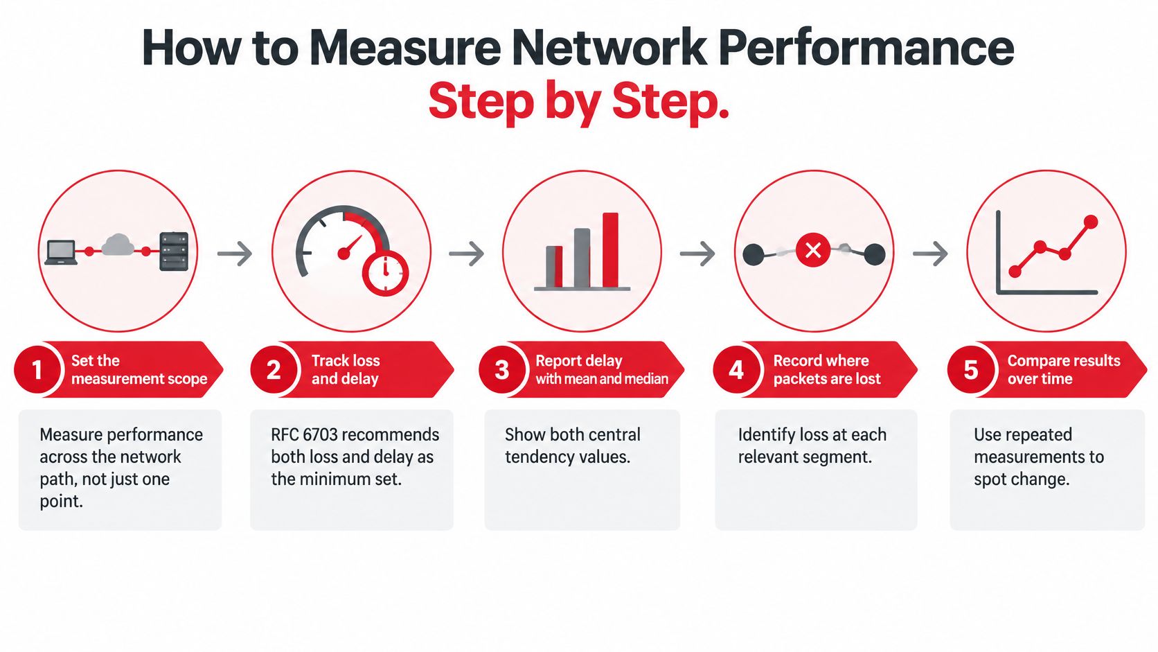
A useful acceptance test measures behavior under changing conditions, not just the highest transfer rate. IETF congestion-control guidance in RFC 5166 treats throughput, delay, packet loss, response to transient events, and stability as distinct evaluation dimensions.
For operational reporting, include both loss and delay, report mean and median delay, and identify missing delay observations as undefined. Otherwise, a delay summary can appear healthy precisely because the worst packets never returned.
Build a controlled test
Define the segment and endpoints. Name the customer device, handoff, transport boundary, or data-center endpoint being tested. Document whether the path includes a firewall, tunnel, wireless hop, or external transit.
Record the idle baseline. Send repeated probes at randomized intervals while the segment is lightly used. For an initial external reachability check, SiteAlive lets you ping a server, but its measurement originates outside your site and won't replace a probe on the affected customer path.
Measure achievable TCP throughput. Use concurrent connections to exercise the available capacity, then test each direction independently. Confirm that the sender, receiver, storage, and host processing aren't limiting the result.
Measure UDP loss at a controlled rate. Record packets sent, packets received, the timeout, and the offered traffic rate. An uncontrolled UDP flood measures how aggressively the test can overwhelm the network, not whether the production service is healthy.
Repeat timing tests under load. Raise traffic toward the planned operating load while keeping latency and loss probes running. A growing gap between idle and loaded delay points toward queue buildup, often described as bufferbloat.
Repeat during the busy period. Test across multiple days and include the hours when users report trouble. A quiet maintenance-window result can't establish busy-hour performance.
Report the distribution. Keep the mean and median, then add agreed tail percentiles and the sample count. Describe the percentile calculation so different tools don't produce apparently conflicting results from the same observations.
Tag every result. Include segment, technology, endpoint, direction, packet size, time, and offered load. Preserve the test configuration so another engineer can reproduce it.
The process works best when scope, loss, delay, and historical comparison remain connected.
Interpret the loaded result carefully
A large loaded-delay increase makes queueing the first hypothesis, not the final diagnosis. Check interface drops, traffic-class counters, shaping policies, and device processing before deciding where the bottleneck sits.
Physical faults and congestion can coexist. Optical receive levels and error counters may identify a damaged segment even when a separate uplink also lacks headroom.
For new construction, retain physical acceptance records alongside service tests. Optical continuity proves something different from application-path performance, and neither should substitute for the other.
If loaded latency rises sharply while idle measurements remain stable, investigate capacity, shaping, and queue management before reopening a splice enclosure or replacing radio equipment.
Monitoring Practices and Tooling
Choose tools by the question they answer. ICMP ping checks reachability and RTT, while traceroute helps identify path changes and boundaries worth investigating.
Don't diagnose forwarding loss from an intermediate traceroute hop alone. Routers may limit responses to diagnostic traffic while continuing to forward production packets normally.
Match collection to the failure
| Tool or Feed | Best Operational Use | Important Limitation |
|---|---|---|
| iperf3 | Controlled TCP throughput and UDP delivery tests | Endpoint limitations can distort results |
| TWAMP-style probes | Repeatable active timing measurements | One-way results require suitable timestamps and synchronized clocks |
| SNMP or streaming telemetry | Interface traffic, errors, discards, and queue state | Polling averages can miss brief bursts |
| NetFlow or IPFIX | Identifying traffic sources and application demand | Flow summaries don't reproduce packet-level timing |
| Syslog and alarm feeds | Outages, route changes, and configuration events | Missing or inconsistent timestamps complicate correlation |
Use a short collection interval during investigations and retain coarser summaries for planning. Keep raw samples where practical, because a smoothed chart can't recover the burst it discarded.
Make the measurements trustworthy
- Synchronize clocks. Use NTP or PTP appropriate to the measurement precision, and monitor clock health rather than assuming synchronization succeeded.
- Stagger probes. Randomized offsets reduce the chance that every test repeatedly aligns with a scheduled task.
- Preserve context. Apply consistent site, circuit, interface, and endpoint labels across metrics and logs.
- Control test overhead. Keep continuous probe traffic modest and schedule intrusive load testing deliberately.
- Alert on actionable behavior. Combine tail-delay breaches with loss, queue state, or user-facing transaction failures instead of paging on every isolated ping spike.
Public crowd-sourced reports help with market comparisons, but they don't establish compliance for a named circuit. Your monitoring must cover the actual contractual boundary and traffic class.
For fiber acceptance, we provide splicing and testing services at Southern Tier Resources, supported by detailed as-built documentation. Those segment records help engineers connect a service-level anomaly to the physical path that needs inspection.
Reading Availability and Utilization Correctly
Allowed downtime for common availability targets
| Availability Target | Downtime per Year | Downtime per Month |
|---|---|---|
| 99.5% | 43.8 hours | 3.65 hours |
| 99.9% | 8.76 hours | 43.8 minutes |
| 99.99% | 52.56 minutes | 4.38 minutes |
These are illustrative arithmetic conversions, using a non-leap-year budget of 8,760 hours and an average monthly budget of 730 hours, not measured service results. Calculate allowed downtime by multiplying the reporting period by the unavailable share.
A calendar-month contract should use the actual duration of that month. An annual allowance doesn't automatically become a monthly allowance, and a provider shouldn't be allowed to erase a bad month by averaging it into a good year.
Define usable service before counting uptime
A physical interface can remain up while the service fails its purpose. If routing breaks beyond the handoff or severe loss prevents a usable call, link-state monitoring alone can overstate availability.
Opensignal's July 2024 U.S. Mobile Network Experience Report gave AT&T a 99.5% mobile-network availability score. That experience-based measure isn't directly interchangeable with contractual uptime for a fixed circuit, so applying it to the downtime table would imply a comparison the measurement doesn't support.
Availability needs an explicit service boundary and failure definition. Without them, the percentage describes the monitoring method more than the user's experience.
Separate outage frequency from total downtime. Frequent brief interruptions can repeatedly reset sessions even when the total unavailable time looks modest.
Read utilization with its queue
Utilization is an average over a measurement interval. It doesn't show whether traffic arrived smoothly or in bursts that temporarily exhausted the output queue.
Consider a hypothetical uplink that looks lightly loaded overnight but approaches saturation during the afternoon. The daily average can look comfortable even though every busy-period call competes with a backup job.
Inspect each direction independently and pair utilization with queue occupancy, discards, and loaded delay. An upstream bottleneck can degrade acknowledgments and interactive traffic even when downstream capacity remains available.
Use a capacity-review trigger, not a universal utilization ceiling. Set it from the point where your own traffic mix produces unacceptable delay or drops, then leave headroom for failover and growth.
Read availability and utilization together. A circuit can remain reachable throughout the month yet become functionally inadequate whenever demand peaks, which calls for a performance remedy rather than an outage-credit argument.
Benchmarks for Wireline, Wireless and Data Center Networks
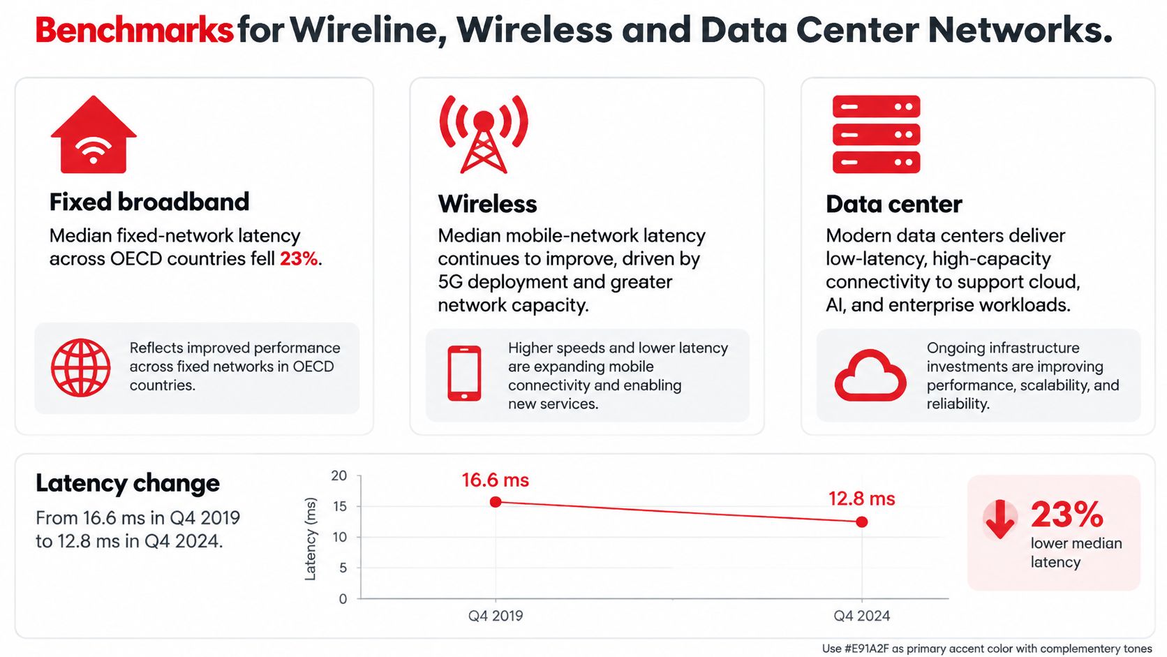
Start with the environment, endpoint, and test method before comparing latency. The OECD's connectivity analysis reports that median fixed-network latency across OECD countries fell 23%, from 16.6 ms in Q4 2019 to 12.8 ms in Q4 2024.
That trend provides context for fixed-access planning, not an automatic pass mark for every broadband circuit. Geography, server placement, and path design still shape the result.
The fixed-network trend is useful when kept within that measurement scope.
Compare like environments
According to Ookla's U.S. Speedtest Connectivity Report, T-Mobile recorded the lowest median U.S. mobile-network latency in the second half of 2024, at 49 ms. That result describes a different population and measurement environment from the fixed-network figures, so it isn't a controlled fiber-versus-mobile comparison.
Metric focus and reference points by network environment
| Environment | Primary Latency Focus | Loss Reference | Secondary Metric to Watch |
|---|---|---|---|
| Wireline fixed broadband | Peak-hour RTT to a consistent endpoint | Set from the application's delivery requirements | Upstream and downstream jitter |
| Mobile wireless | Median and tail delay under representative radio load | Establish by service path and radio conditions | Availability and scheduling delay |
| Data center interconnect | RTT across the named interconnect and traffic class | Set a strict delivery objective from baseline and workload needs | Microburst-related jitter, discards, and interface errors |
For wireline access, test beyond the nearest convenient speed-test server when the application lives elsewhere. A clean access segment doesn't establish clean transit to a cloud workload.
For wireless, record radio conditions, scheduling context, and mobility state alongside network measurements. Comparing a stationary device under light load with a moving device at a busy site won't isolate infrastructure quality.
Judge interconnects by workload behavior
For data-center interconnects, path length and topology establish the delay floor. The more useful operational question is often whether bursts introduce discards or unstable delivery across an otherwise short, predictable path.
Correlate queue telemetry with application traffic patterns. A storage replication workload, distributed service, and bulk migration can stress the same interconnect differently even when their average traffic rates look similar.
There isn't a reliable universal loss ceiling or metro-latency target in these public benchmarks for every data-center workload. Treat that as a specification gap to close with acceptance testing, not an invitation to copy a convenient number.
A benchmark tells you where to investigate. Your service baseline tells you whether the measured path has changed and whether users' requirements are still being met.
Mapping Metrics to SLAs and KPIs
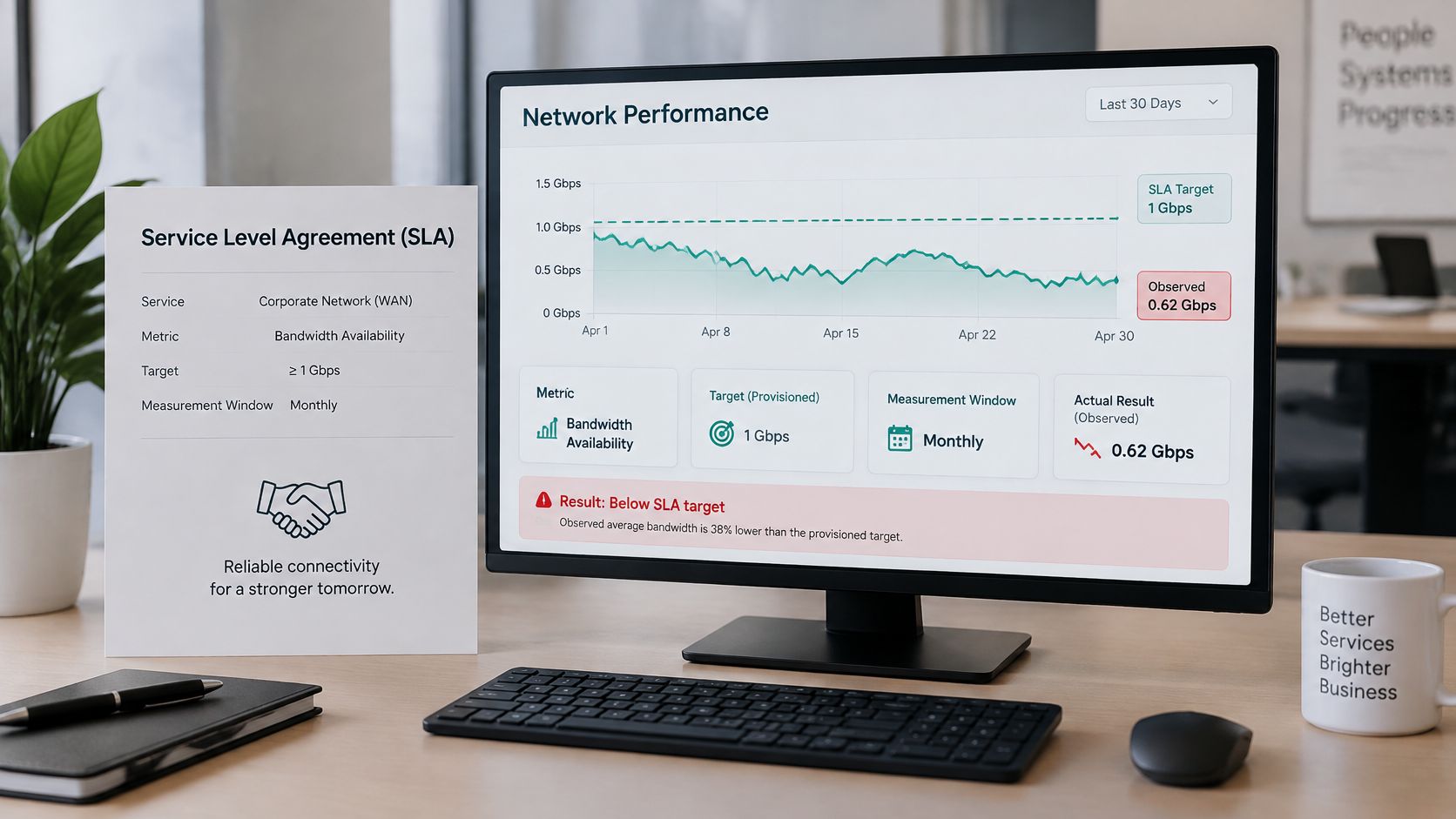
A provisioned capacity is a design input. An observed service outcome is what the customer receives at the agreed boundary, under the agreed conditions.
Write latency commitments with a named metric, measurement point, percentile, and covered share of sessions. Include direction, traffic class, and load conditions so a provider can't satisfy an application requirement with a favorable measurement elsewhere.
Contract for the service path
Use boundaries such as the radio access network, transport handoff, core exit, or application endpoint. A transport-only guarantee shouldn't be presented as an end-to-end application promise.
A 2025 network-performance study treats performance as use-case-specific and evaluates predicting delay, jitter, and loss. The operational implication is to define the service objective before choosing the assurance metric, rather than applying the same commitment to unrelated workloads.
Percentile coverage and session coverage aren't interchangeable. A packet-delay percentile across all observations can conceal a small group of consistently poor sessions, so report session success separately.
A dashboard should distinguish the contractual limit from the actual result.
Translate commitments into operational KPIs
- Latency. SLA clause: the agreed tail RTT must remain below the contracted limit between named endpoints under specified load. KPI: compliant measurement windows and affected sessions.
- Jitter. SLA clause: per-flow packet-delay variation must remain within the agreed application tolerance. KPI: variation breaches by direction, traffic class, and service.
- Loss. SLA clause: loss must stay below the contracted rate, with a separate rule for damaging bursts. KPI: interval loss, consecutive-loss events, and affected sessions.
- Availability. SLA clause: usable service must meet the agreed monthly target at the defined boundary. KPI: qualifying downtime, incident count, and restoration duration.
- Utilization. Operating clause: capacity review begins when the agreed peak-demand trigger is reached. KPI: headroom, queue growth, and time spent beyond the trigger.
These are clause structures, not ready-made thresholds. Populate them from baseline measurements, application requirements, and realistic recovery behavior.
Keep utilization primarily as a planning KPI unless the contract explicitly guarantees headroom. Customers need usable service, while operators need flexibility to manage capacity efficiently.
Before signing, agree on probe ownership, sample validity, reporting windows, planned-maintenance treatment, and exclusions. Also define how overlapping failures count, how disputes are reproduced, and whether a failed session can be excluded merely because it produced no timing result.
Troubleshooting Real Cases With a Reporting Template
Symptom, likely cause and first metric to check
| Symptom | Likely Cause | First Metric to Check |
|---|---|---|
| Pages load slowly despite a high speed test | Queueing increases delay under load | Idle versus loaded latency |
| Calls sound choppy or drop words | Jitter spikes or loss bursts | Per-flow jitter and loss by interval |
| Speed drops only at peak hours | Demand approaches the constrained segment's capacity | Peak-hour utilization per interface |
| Frequent short outages | Link instability, route changes, or repeated recovery | Outage count and downtime per month |
| Intermittent errors on one segment | Fault on a specific path or device | Metrics tagged by segment and endpoint |
Treat this table as an investigation order, not a diagnosis. Slow pages can also come from DNS, server processing, or application dependencies, so confirm that network timing changes with the complaint.
Work the evidence before choosing the repair
Consider a hypothetical business site where calls freeze late in the working day while throughput tests remain healthy. Idle timing is stable, but delay rises sharply when the upstream link carries sustained traffic.
Start probes on both sides of the customer gateway and at the provider handoff. Compare their timing with interface queues, discards, and application flows during the reported failure window.
If the delay first appears at the constrained uplink, queue occupancy rises with a scheduled transfer, and physical error counters remain clean, queueing is the leading diagnosis. That evidence doesn't justify calling the fault a bad fiber splice, nor does it yet prove provider oversubscription farther upstream.
Test a targeted remedy. Reschedule the bulk transfer, correct shaping to match the actual service rate, or apply queue management and a bounded priority class for interactive traffic.
Prioritization trades waiting time between classes; it doesn't create capacity. If legitimate demand continues to fill the link, add capacity rather than indefinitely depriving other applications of service.
Retest discipline: Change a defined variable, reproduce the original load, and verify the user-facing service as well as the network counters.
Repeat the test during the same busy conditions. A quiet-period result after a configuration change doesn't establish that the afternoon problem is resolved.
Keep a report engineers can act on
- Reporting period and identity. Record the site, circuit, service boundary, endpoints, direction, and configuration version.
- Delay distribution. Include median and agreed tail latency at idle and under load, with sample counts and missing observations.
- Delivery quality. Record per-flow jitter, loss by interval, burst events, and relevant traffic classes.
- Continuity. List usable-service availability, incident count, downtime, and restoration details.
- Capacity and condition. Include peak utilization, queue behavior, discards, interface errors, and optical or radio indicators where relevant.
- Diagnosis and action. Separate confirmed causes from hypotheses, then identify the owner and change made.
- Retest outcome. Preserve comparable before-and-after results and confirm whether the original application complaint stopped.
Publish the report monthly and after material changes. Keep unresolved hypotheses visible rather than converting them into facts through repetition.
The strongest network performance report connects a symptom to a segment, an observed failure mechanism, and a verified repair. That's what separates a healthy network from one that merely passes a speed test.
We provide engineering, construction, splicing, testing, and maintenance for wireline and wireless networks, along with data-center infrastructure fit-outs. Visit Southern Tier Resources to discuss your deployment or maintenance scope and the segment-level testing and documentation needed to support dependable network performance.