Network jitter is the variation in delay between successive packets, not the delay itself. If every packet experiences exactly the same delay, jitter is zero, even when the connection feels slow.
You're on a video call, voices keep breaking up, and the bandwidth dashboard looks healthy. The average latency looks reasonable too, so the project team asks whether the circuit needs upgrading. Before authorizing more capacity, check whether packets arrive consistently, and whether the dashboard measures the same path, traffic, and time window as the application.
What Network Jitter Means in Plain Terms
Network jitter is variation in packet delay, not simply a slow connection.
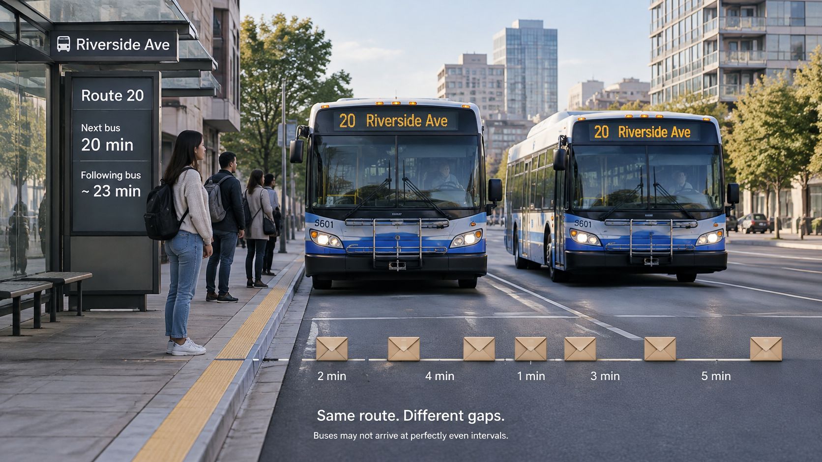
Think about buses serving a familiar route. A bus that takes a predictable amount of time lets passengers plan their journeys. A service that alternates between quick trips and long delays makes planning harder, even if its average journey time looks respectable.
Packets behave similarly. The sender produces a stream, but the network doesn't necessarily preserve its spacing. A packet may pass through an empty router queue while the next waits behind competing traffic.
The bus analogy makes that irregular delivery easier to visualize.
Why packet spacing matters
A voice receiver must play audio continuously, not merely collect packets eventually. When delivery becomes uneven, the receiver has to absorb that variation or decide what to do when the next piece of audio isn't ready. Video meetings, cloud games, and industrial control flows also depend on timely delivery.
The International Telecommunication Union's buffer-model guidance distinguishes constant delay from delay variation: identical delay for every packet means zero jitter, regardless of the absolute delay. In packet networks, packet delay variation, or PDV, is often the more precise technical term.
That distinction prevents a common misunderstanding. A stable path can still be too slow for an application, while an otherwise responsive path can deliver packets too unevenly for smooth playback. Neither condition tells you everything about the other.
A jitter number needs a measurement definition
Jitter isn't a single universally calculated quantity. A tool might summarize changes between successive packets, maintain a smoothed estimate, or report the spread between the largest and smallest delays in an observation window.
The window matters because a brief queue buildup may dominate a short measurement but become almost invisible inside a much longer average. An idle-path test can also miss the variation users experience during production traffic.
Before using a jitter result, identify:
- Endpoints: Where did measurement start and stop, and in which direction?
- Sample window: When were packets observed, and how were they spaced?
- Calculation method: What mathematical operation produced the reported value?
Without those details, comparing jitter numbers is like comparing journey times without knowing the route.
How Jitter Differs From Latency and Packet Loss
| Metric | What It Measures | Unit | Typical Cause | Example |
|---|---|---|---|---|
| Latency | Time one packet takes to cross the network | Milliseconds | Distance, propagation, processing, and queuing | A packet arrives later because the route is longer |
| Jitter | Variation in packet delay | Milliseconds, or media timestamp units before conversion | Changing queues, route transitions, retransmissions | Adjacent packets experience different waiting times |
| Packet loss | Share of transmitted packets that don't arrive within the measurement definition | Percentage | Congestion drops, faulty links, exhausted buffers | Missing packets divided by transmitted packets, expressed as a percentage |
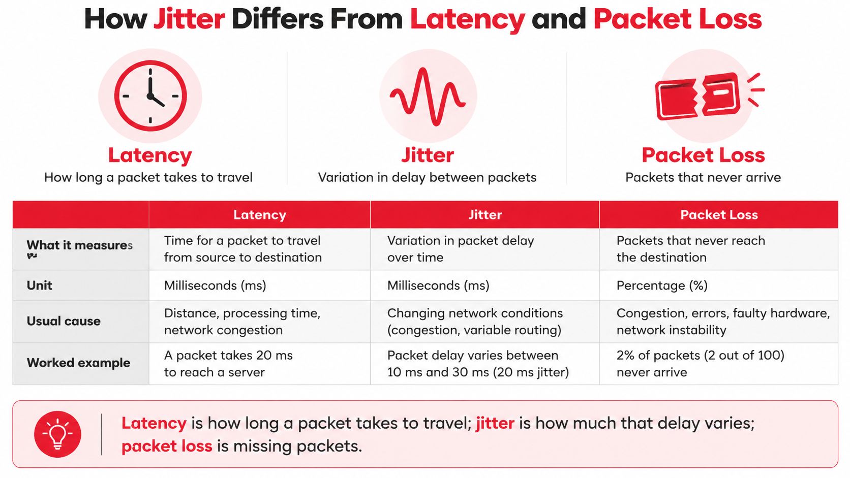
Latency describes the trip time. Jitter describes how uneven those trips are. Packet loss describes packets the receiver doesn't get, subject to the test's rules for declaring a packet missing.
Consider a hypothetical voice flow sharing an uplink with a file transfer. Some voice packets cross while the queue is empty; others arrive during a burst and wait. Every packet might eventually arrive, but the audio receiver still has an irregular stream to handle.
The distinctions are easier to keep separate when viewed side by side.
What the combination tells you
The IETF's RTP specification explains that packet loss tends to track persistent congestion, while jitter can reveal transient congestion before packets are dropped. That's a diagnostic relationship, not a claim that congestion causes every lost packet.
If average latency is within the application's target and measured loss is negligible, but calls still break up, investigate timing variation next. Correlate the application's troubled periods with queue occupancy, route events, and receiver playout behavior. Also check endpoint performance rather than assuming the transport network is responsible.
An acceptable average doesn't prove acceptable delivery. A summary can combine long quiet periods with short bursts that users notice immediately.
Compare distributions, not unrelated averages
Inspect a time series and relevant percentiles alongside the maximum. Keep the measurement window visible, since a maximum from an extended observation period isn't directly comparable with a maximum from a brief test.
Be precise about what a percentile describes. A percentile of packet delays is not the same quantity as a percentile of per-interval jitter estimates. Both may help operations teams, but labeling them as “jitter” makes troubleshooting harder.
Low jitter alone also isn't a universal pass. The application can still suffer from excessive trip time, missing packets, or endpoint stalls.
Report latency, jitter, and packet loss together, with the endpoints, direction, observation window, and calculation method attached.
What Causes Jitter Across Wired and Wireless Networks
The immediate cause is usually a changing amount of time spent waiting, processing, or recovering from transmission problems. Finding the responsible segment requires matching the timing pattern to an operational event, rather than identifying the busiest interface.
| Cause | Where It Appears | Typical Signature | First Check |
|---|---|---|---|
| Bufferbloat | Modems and routers with oversized queues | Delay and jitter rise during sustained transfers | Ping during a large upload |
| Congestion | Shared links at peak periods | Variation increases with demand; loss may follow | Interface utilization over time |
| Queuing and scheduling | Switches and routers | Real-time traffic waits behind bulk traffic | Queue depth and drops by traffic class |
| Clocking and synchronization | Mobile backhaul and TDM-to-packet gateways | Timing offsets or buffer underruns | PTP or SyncE lock status |
| Wireless retransmissions | Microwave, cellular, and Wi-Fi links | Delayed packet clusters around radio impairment | Retry counters and signal-level logs |
| Last-mile variation | DSL, cable, and shared fixed wireless | Changes follow local demand | Repeat the test from a wired port at different demand periods |
| Route changes | Failover paths and peering transitions | A step change in the delay baseline | Compare path observations before and after the event |
Wired networks and changing queues
Bufferbloat occurs when a device retains enough queued traffic to create excessive waiting time. During a sustained upload, a modem or router may continue accepting packets while the outbound link drains more slowly. Interactive traffic then waits behind traffic that doesn't need immediate delivery.
Start a continuous ping before a controlled upload and keep it running throughout. If round-trip delay rises with the transfer and recovers afterward, inspect the bottleneck's queue management and shaping configuration. The test identifies a load-related symptom, not necessarily the exact device.
Congestion and scheduling require a closer look at individual queues. An interface average can look comfortable while short bursts fill a queue, and aggregate utilization won't show whether voice traffic receives the intended treatment. Examine class counters, scheduler configuration, and drops together.
Timing problems need separate treatment. In timing-sensitive transport, loss of synchronization can affect clock recovery and buffer behavior without resembling ordinary bandwidth congestion. Check lock transitions and offsets rather than treating every periodic disturbance as an IP queue problem.
Wireless recovery and path transitions
Radio links introduce additional variables. Wi-Fi contention and retries can delay packets, while fading or interference can reduce a microwave link's usable capacity. When incoming traffic exceeds that reduced capacity, queues can build even though offered traffic hasn't changed.
Route changes produce another signature: a new delay baseline rather than random variation around the old one. Correlate the transition with routing logs, because traceroute alone may not expose every forwarding change.
Transient events deserve their own monitoring: the Internet Society's 2025 Internet-edge measurements found that approximately 4% of all observations exhibited latency spikes at least two orders of magnitude greater than those reported in recent prior work. That finding supports inspecting spikes directly rather than relying only on a daily average.
How to Measure Jitter With a Sample Calculation
- Choose the endpoints and path. Record source, destination, direction, access medium, and traffic class. Decide whether you need application-to-application coverage or isolation of a particular network segment.
- Choose a representative packet profile. Match packet size, spacing, protocol, and priority treatment to the service you're evaluating.
- Include contrasting operating conditions. Measure during quiet periods, busy periods, and controlled load where it's safe to do so.
- Retain packet-level timing. Preserve sequence information, timestamps, loss, and relevant network events rather than keeping only a final average.
- Apply a named calculation. State whether the result is successive-delay variation, an RTP smoothed estimate, or another defined metric.
- Report the distribution and exceptions. Include the agreed percentile, extremes, observation window, and application symptoms.
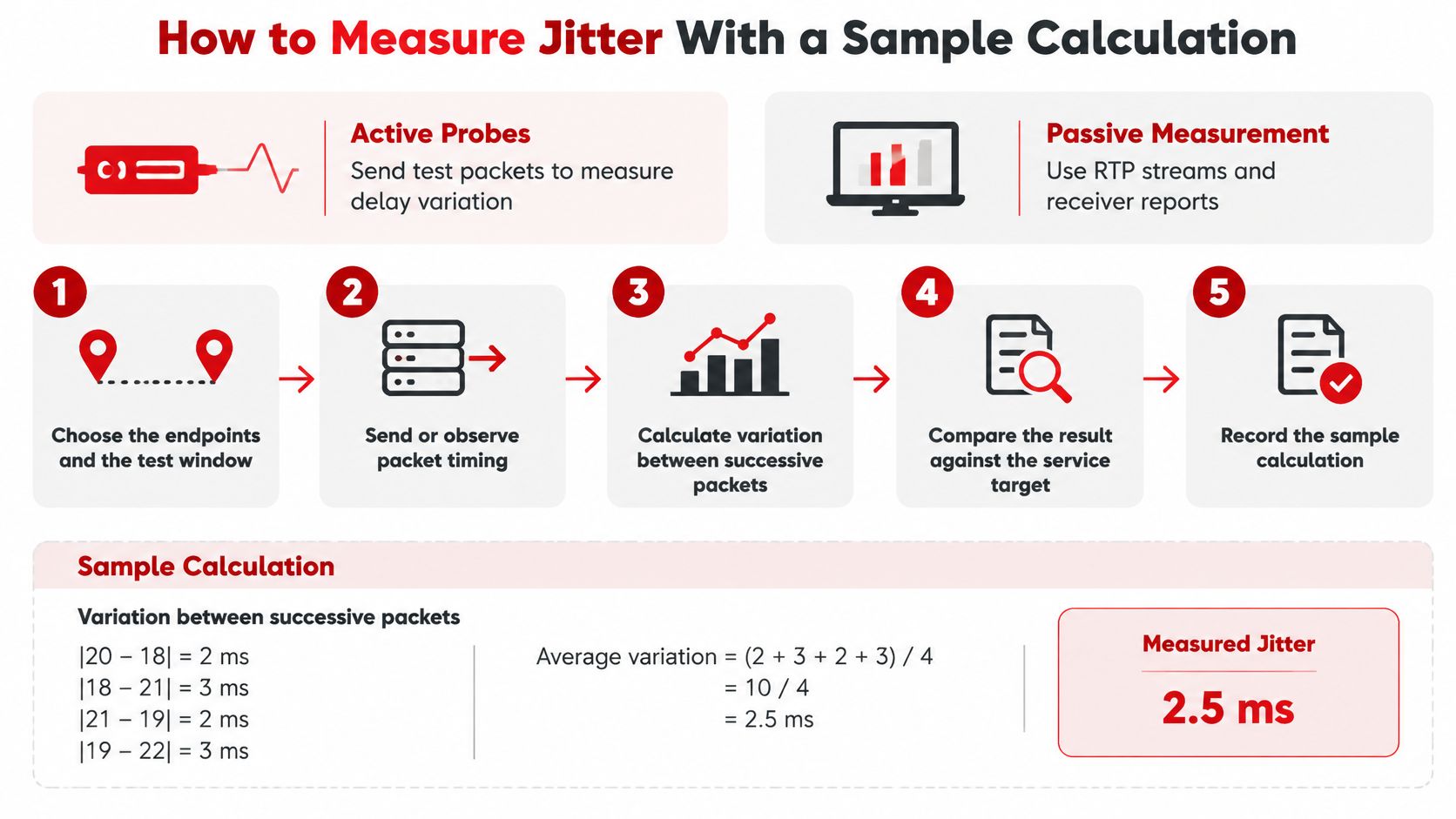
The measurement workflow should make the calculation traceable to actual packet timing.
Choose active or passive measurement
Active probes generate test traffic between selected endpoints. Use ping and traceroute for initial reachability and path checks, iperf3 in UDP mode for controlled traffic testing, and TWAMP where supported for two-way measurements between managed endpoints.
Passive measurement examines existing traffic. For voice or video, Wireshark's RTP Stream Analysis and receiver reports can help connect transport timing with an actual media session. Capture placement matters: observing a stream before a congested segment won't describe what its receiver experiences afterward.
| Test Purpose | Packet Pattern | Duration | Pass Signal |
|---|---|---|---|
| Quick link check | ICMP probes with documented spacing | Long enough to establish a repeatable baseline | Stable baseline without unexplained excursions |
| Voice readiness | Continuous UDP matching the deployed voice profile | Covers representative call activity | Meets the service's defined metric without playout underruns |
| Under-load test | Voice-profile traffic alongside controlled bulk transfer | Covers queue buildup and recovery | Meets the agreed target throughout the load condition |
| Busy-hour probe | Continuous application-shaped UDP probes | Covers the complete relevant demand cycle | Peak-period results satisfy the documented acceptance rule |
These are test profiles, not universal thresholds. Put the actual duration, packet interval, and pass criterion in the test plan before running them.
Calculate a transparent example
Consider a hypothetical set of packet delays:
20, 23, 19, 31, 22 ms
The absolute differences between successive delays are:
3, 4, 12, 9 ms
The mean absolute successive-delay difference is therefore:
(3 + 4 + 12 + 9) ÷ 4 = 7 ms
The maximum-minus-minimum delay spread is:
31 − 19 = 12 ms
Those results describe the same hypothetical packets using different calculations. Neither should be presented as interchangeable with an RTP receiver's smoothed jitter estimate.
The IETF's RFC 3550 defines the RTP update as J(i) = J(i−1) + (|D(i−1,i)| − J(i−1))/16, and explains that at an 8,000-Hz media clock, 80 timestamp units equal 10 milliseconds.
Using the hypothetical differences above, starting at zero gives:
J = 0 + (3 − 0)/16 ≈ 0.19 ms
Applying the next hypothetical difference gives:
J ≈ 0.19 + (4 − 0.19)/16 ≈ 0.43 ms
The smoothing retains history, which explains why it doesn't immediately equal the arithmetic average. RTP's spacing difference also accounts for sender timestamps, rather than treating receiver arrival spacing alone as network variation.
Keep direction and clocks explicit
Ping measures round-trip time, so its variation includes outbound travel, return travel, and endpoint handling. It doesn't isolate forward-path jitter.
One-way delay measurements need a trustworthy relationship between endpoint clocks. Record synchronization quality, and don't compare a round-trip probe result with a one-way application metric.
For a complementary visual walkthrough of testing, use the video below.
Acceptable Jitter Limits for Each Service
| Service | Jitter Target | Latency Target | Notes |
|---|---|---|---|
| VoIP | Set against the deployed receiver and playout behavior | Application's agreed conversational-delay budget | Late arrivals can cause choppy audio when buffering can't compensate |
| Video conferencing | Validate with the deployed conferencing platform | Agreed interactive meeting target | Check freezes, audio continuity, and loss together |
| Cloud gaming | Validate against the game and streaming implementation | Agreed end-to-end interaction budget | Rendering, encoding, transport, and decoding all matter |
| Cloud interconnect, dedicated | Contract-defined metric and interval | Route-specific SLA requirement | Confirm direction, percentile, exclusions, and measurement points |
| Ultra-reliable low-latency services at the edge | Use the application-specific engineering target | Use the corresponding round-trip or one-way requirement | A study target isn't a general service standard |
There's no defensible universal table that assigns every application a single pass/fail jitter value. The receiver's buffering, the application's deadline, and the calculation method all affect what a reported number means.
For voice, examine the actual playout behavior. A receiver may absorb arrival variation successfully, but doing so can increase playback delay. Passing the network metric while users struggle to take turns speaking isn't a successful outcome.
Different applications have different deadlines
Video conferencing combines audio continuity with video presentation and synchronization. A receiver may hide a late video update differently from a missing section of speech, so transport measurements should be paired with application diagnostics.
Cloud gaming adds an input-to-display deadline. The operator needs to assess the network alongside game-engine behavior, frame delivery, encoding, and decoding rather than judging the session from access-link jitter alone.
Dedicated cloud interconnects require careful contract reading. Confirm whether the SLA measures a mean, a percentile, or another statistic, and whether it covers the path your workload uses. A provider-edge measurement doesn't automatically represent a host-to-host experience.
Use narrow targets only within their scope
A 5G edge-slicing study used engineering targets of jitter below 2 ms and RTT below 20 ms, with observed packet jitter generally within 0–1.5 ms in its tested scenarios. Those figures belong to that tested design and use case, not to every wireless deployment.
The practical lesson is architectural. Where the application needs highly predictable timing, teams may need to address edge placement, radio scheduling, transport paths, and processing placement together. A faster access circuit can't compensate for every source of end-to-end delay variation.
Acceptance rule: Choose the application outcome first, then define the jitter metric, observation window, and test conditions that demonstrate it.
When a service exceeds its target, inspect RTT and loss at the same time. Buy capacity when the measurements establish a capacity problem, not just because someone has labeled an application complaint “jitter.”
Mitigation Strategies for Design and Operations
Start at the queue that introduces the waiting time. Increasing a receiver buffer can conceal some symptoms, but correcting transport behavior avoids adding unnecessary application delay.
Priority queuing gives time-sensitive traffic preferential service. For managed voice, DSCP EF is a common classification choice, but the marking must map to the intended queue across the administrative boundaries you control. Unrestricted priority traffic can starve other classes, so admission control and policing matter.
Active queue management addresses excessive queue persistence. Consider fq_codel, CoDel, or PIE where supported, and verify behavior on the actual bottleneck rather than assuming a feature checkbox proves correct operation.
| Mitigation | Where to Apply | Effect on Jitter | Trade-off |
|---|---|---|---|
| Priority queuing with voice classification | Access and core routers | Reduces waiting behind bulk traffic | Other classes wait longer; priority traffic needs control |
| Active queue management | Edge devices, CPE, routers | Limits persistent queue buildup | Requires suitable configuration and validation |
| Shaping below effective bottleneck capacity | Network edges | Moves queue control to a managed device | Reserves headroom instead of using all nominal capacity |
| MPLS-TE or segment routing | Managed core network | Can avoid congested or unsuitable paths | Adds policy and control-plane complexity |
| PTP and SyncE | Timing-sensitive transport | Addresses synchronization-related impairment | Requires an engineered timing architecture |
| Percentile and event-based alerting | Monitoring systems and probes | Exposes service-affecting excursions | Needs consistent definitions and appropriate probe coverage |
Control the bottleneck, not just the marking
A shaper should reflect the effective service rate, including relevant encapsulation and variable-link behavior. If it's configured above the actual bottleneck, the uncontrolled downstream queue can still accumulate traffic. If it's too conservative, the operator sacrifices usable throughput unnecessarily.
Test QoS under contention. Verify classification counters, queue occupancy, and drops while representative real-time traffic competes with a bulk transfer. Don't assume DSCP markings survive a carrier handoff, tunnel, firewall policy, or customer-premises device.
Traffic engineering is useful when a better path exists and the forwarding policy can select it consistently. It isn't a substitute for capacity planning, and frequent steering changes can introduce their own operational problems. Validate both normal and failure paths.
Engineer timing and monitor application impact
PTP and SyncE solve different timing needs and should be selected accordingly. Choose boundary or transparent clock behavior where the timing design calls for it, and monitor source changes, lock state, and offsets. Adding timing features indiscriminately won't correct ordinary IP congestion.
Receiver jitter buffers remain useful, but tune them against conversational or interaction delay. A larger buffer may reduce underruns while making a meeting feel less responsive. Evaluate both outcomes during the same test.
Finish with operational ownership:
- Capacity planning: Track busy-period demand, traffic mix, and growth against the weakest segment.
- Correlated alerting: Combine jitter excursions with utilization, queue drops, route changes, and radio events.
- Change validation: Repeat the representative service test after scheduler, routing, firmware, or access changes.
- Incident evidence: Preserve the underlying time series so engineers can distinguish a sustained problem from a brief transition.
Backhaul Design and Fiber Versus Microwave Choices
| Consideration | Fiber | Microwave | Jitter Implication |
|---|---|---|---|
| Propagation delay | Set by optical path length and equipment | Set by radio path length and equipment | Fixed propagation delay isn't itself jitter |
| Capacity stability | Not subject to radio fading | May change with fading, interference, or modulation | Reduced capacity can increase queuing |
| Variation sources | Queuing, equipment faults, reroutes | Queuing, radio impairment, recovery behavior | Different mechanisms need different telemetry |
| Deployment constraints | Duct access, permits, civil works | Site access, alignment, spectrum, path clearance | Construction choices affect topology and test access |
| Failure behavior | A cut may trigger a different route | A fade may reduce rate or trigger protection | Evaluate both the transition and the resulting path |
Choose backhaul using its operating envelope, not just its nominal rate. Fiber and microwave can both support demanding services when the design accounts for bottlenecks, protection behavior, and timing requirements.
Fiber avoids radio-induced capacity changes, but a fiber route still contains active equipment, aggregation queues, and protection mechanisms. A well-built optical segment doesn't guarantee predictable application delivery if upstream aggregation is oversubscribed.
Microwave can serve routes where civil construction is difficult, but the design needs to account for usable capacity during degraded radio conditions. A link that carries normal demand comfortably at its highest modulation may become a bottleneck when conditions worsen.
Design around the degraded state
Keep aggregation paths straightforward. Each forwarding and scheduling stage adds another place where packets can encounter competing traffic, so review the entire chain rather than approving each hop independently.
For microwave, align traffic policies with adaptive capacity. Protect critical traffic when the radio reduces its rate, and define how lower-priority traffic is constrained. A policy based only on clear-weather capacity won't necessarily preserve interactive performance.
A hypothetical multi-hop microwave chain illustrates the issue. During a storm, a hop reduces capacity while traffic continues arriving from upstream at the previous rate. The resulting queue can disrupt a voice flow even though the route's long-term throughput report looks acceptable.
Test protection as a service condition
Hybrid designs can use microwave and fiber to provide alternate connectivity, but the backup path needs its own acceptance criteria. Confirm that traffic classification, timing distribution, and bottleneck control remain valid after failover.
A fiber cut may move traffic to a longer route with a different baseline delay. That steady new baseline isn't ongoing jitter by itself, although the transition can contribute to variation within the observation window. Keep route-state timestamps with performance records so operators can distinguish the transition from continuing instability.
Use these design checks:
- Aggregation headroom: Evaluate shared uplinks under combined demand and failure conditions.
- Timing placement: Confirm how timing reaches remote equipment when the preferred path fails.
- Radio resilience: Review fade margin, interference exposure, and capacity-dependent policies.
- Protection testing: Measure the application during switchover, not only after routing stabilizes.
Confirm Jitter Limits Before Accepting the Network
Don't accept a link solely because it passes an idle test. Acceptance should demonstrate the agreed service behavior under representative load, using a measurement definition both the construction team and operations team can reproduce.
The acceptance record should connect physical infrastructure, forwarding behavior, and application performance. A clean optical test or successful radio alignment is necessary evidence for its layer, but neither substitutes for an end-to-end packet test.
- Record the pre-cutover baseline. Measure from the agreed endpoints in each required direction, and save the packet profile, tool version, clock status, and path details.
- Run readiness and load tests. Use representative application traffic alongside controlled background demand, including queue buildup and recovery.
- Observe the demand cycle. Keep probes running through relevant peak periods and scheduled background jobs.
- Verify timing where required. Check synchronization state and offsets throughout timing-sensitive paths.
- Resolve or document exceptions. Attach timestamps, endpoints, observation windows, calculation methods, and application impact to each deviation.
- Hand over reproducible records. Include as-built plans, probe locations, thresholds, alert rules, and raw or exportable test results.
The engineer receiving the network needs enough detail to repeat the acceptance test later.
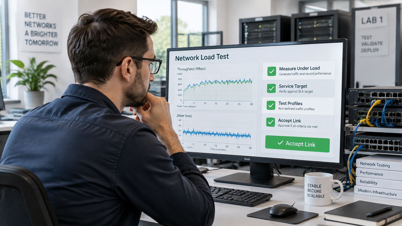
Test construction quality before access becomes difficult
Inspect and test fiber segments before closing access to work areas. For radio paths, complete path-clearance and fade-margin checks during design, then validate installed alignment and performance before acceptance. Don't defer accessible construction checks until a service complaint forces a return visit.
At Southern Tier Resources, we serve networking and data firms with telecom solutions. For a project team, that makes clear handover requirements important: operations needs documentation that connects the built infrastructure to the endpoints and conditions used for performance testing.
Write the acceptance definition into the build contract. Specify the service target, direction, packet profile, observation window, calculation method, required load conditions, and treatment of failures or excluded samples. Require the test records as a deliverable, with an owner assigned to resolve exceptions before sign-off.
We provide telecom solutions for networking and data firms, including fiber construction for broadband networks. Visit Southern Tier Resources to discuss your infrastructure project and bring its jitter measurement, testing, and handover requirements into the planning conversation.